[NMR analysis blog] Basics on Arrayed-NMR Data Analysis (Part III): Extracting and calculating useful NMR

[nmrlearner]

Basics on Arrayed-NMR Data Analysis (Part III): Extracting and calculating useful NMR related molecular information

After the basic introductory posts on arrayed NMR experiments, it’s now time to get some action and see how to extract relevant information from these experiments and calculate useful NMR related parameters such as diffusion, relaxation times, kinetics constants, etc.

Actually, in this post I will cover the first case, that is, the analysis of PFG experiments to calculate diffusion coefficients. The reason for this is twofold: (1) I have a nice PFG data set whilst the quality of the relaxation experiments I currently have access to is quite poor (if any of you have any good relaxation data and can send them over, I would be very grateful) (2) The current version of Mnova has been optimized to handle PFG experiments fully automatically whilst some simple manual intervention is needed when working with other arrayed-like NMR experiments. However, I would like to emphasize that, for example, relaxation experiments are already fully supported in the current version of Mnova, although it is necessary to enter the time delays manually in the program (this is very simple, btw). Automation of relaxation experiments is already possible with alpha versions of Mnova.

This is how a PFG experiment can be analyzed with Mnova with the Data Analysis module (for your information, Mnova includes a DOSY-like processing algorithm based on a Bayesian Algorithm. See this http://mestrelab.com/dosy.html and this http://nmr-analysis.blogspot.com/200...nder-hood.html for more information):

Once the arrayed spectra has been loaded into Mnova, issue menu command Analysis/Data Analysis. The so-called Data Analysis widget will popup. This will be the central control panel (see figure below) for anything related to the analysis of arrayed experiments.


Its operation is very simple. The first thing you have to do is click on the New button. As a result, Mnova will populate the X-Y Table with some initial values (as described in a moment) and create a new item, the so-called Data Analysis Plot. This new item will display the values from the X-Y Table which in general are the values extracted from the arrayed spectra, both experimental (Y) and fitted (Y’).



The X-Y Table
This table is composed by one X column, X(I), one or several Y-columns (Y, Y1, Y2, etc) to hold the experimental values extracted from the arrayed spectra and one or several Y’-columns which hold the fitted values of their Y counterpart columns.


X-Column
When the table is initialized, in the case of PFG experiments the X-column is populated with the Z values from the Diffusion table, that is, the gradient strengths scaled by taking into account the constants from the selected Tanner-Stejskal model. In the case of a relaxation experiment, the X column will contain the time delays. Of course, it is possible to change the contents of the X-column by following any of these methods:

• Manual editing of the individual cells

• Copy & paste from a text file. For example, you can put the values for the X-column into a text (ASCII) file and then paste its contents into the table. To do that, just right click on the first cell you want the paste action to start from.

• Enter a formula into the Model cell. Double click on the X(I) model cell (1) and then enter the appropriate equation to populate the X column (2). For example, if you simply enter I, the X column will be filled in with numbers 1, 2,3, etc. If you enter a formula like 10+25*I, the X column will be filled with numbers 35,60, 85, etc.

Y-Column
In all cases, when the table is initialized, the Y-column is automatically filled in with values 1,2,3, etc. The purpose of this column is to hold the experimental values from the arrayed experiment. For example, in the case of a PFG experiment, it may contain how the intensity (or integral) of a given peak (or set of peaks) evolves as the applied pulse field gradient changes. Likewise, in the case of T1/T2 experiments, this column will show the relaxation profile of a given resonance (or set of resonances). So the question is: how to populate the Y-column with actual information from the spectra?


This is again very easy. There is a graphical way (mouse driven) and a manual one. Let’s start with the graphical method:

• Graphical Selection: Click on the ‘Interactive Y Filling’ button (see red-highlighted button in the image below). After doing this, the cursor will change into an integral shaped cursor expecting you to select the region from where you want the integrals to be extracted across all the subspectra in the arrayed item. After the selection is done (see figure below), all the integrals will be placed in the Y column and those values will be displayed in the X-Y plot as green crosses (note: the shape, color, etc of these crosses can be customized from the X-Y plot properties).

• Manual selection: if you take a closer look at the Data Analysis table in the figure above, you can appreciate that once the integral region has been selected, the program shows the following text: Integral(4.752, 4.907). This means that we have selected an integral covering that range. This value can be edited manually so that you can specify the limits by simply editing that cell.

Y’-Column
The Y’ column is reserved for the fitted values assuming a particular theoretical model (e.g. a exponential decay). In this particular case, as we are dealing with PFG experiments, we will be interested in the calculation of the Diffusion coefficients and thus, our fitting model could be a mono-exponential decay (multi-exponential decays can also be handled with this module, but I will not address this problem in this post). The process is very simple:

First click on the Y’(X) cell and then on the small button with 3 points as indicated in the figure below.


This will launch a dialog box with powerful fitting capabilities.


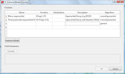
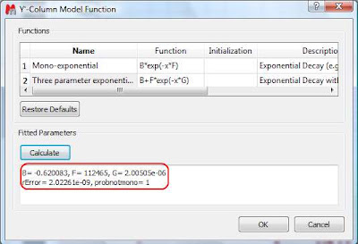
This dialog provides two predefined functions useful for fitting mono-exponential data (such as PFG and Relaxation NMR experiments) using either a 2- or a 3-parameter fit. Furthermore, this dialog offers the possibility to enter user customized functions. As this post is already taking too much space, I will leave the details on data fitting for the next post. For the time being, suffice to say that if your problem regards mono-exponential functions, just select any of the 2 predefined functions in the dialog box and click on the Calculate button. Mnova will immediately compute the optimal values, returning these optimal values as well as the fitting error) and the probability that the acquired series follows the chosen monoexponential model.



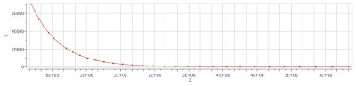
Finally, after closing the dialog, it will populate the Y’ column and the X-Y will be updated with the fitted curve (Red line in the figure below).


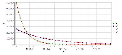
One nice feature of the Data Analysis module is its ability to handle multiple series. For example, it’s possible to analyze the decay of several resonances within the same experiment. In order to do that, just click on the (+) button to add a new series and repeat the same process to select the desired resonance range and fit the values. For example, in the figure below I’m showing two curves with different decay rates.

In my next post I will cover some more details about the different methods available to select the intensities/integrals from the spectra and some basic points on the fitting algorithm.
BTW, you can download the full PFG data set used in this post



More...

Source: NMR-analysis blog